Q7(a) Expectation Maximization algorithm [5]

Answer

A Gaussian mixture models a population using K Gaussian components. A hidden component label says which component generated a sample. The labels are not observed, so the likelihood sums over all possible components.

LaTeX: p(x_i\mid\theta)=\sum_{k=1}^{K}\pi_k\mathcal N(x_i\mid\mu_k,\Sigma_k),\quad \pi_k\geq0,\quad\sum_k\pi_k=1

Step 1. Form the observed-data log likelihood

For independent observations multiply their densities; taking the logarithm turns the product over observations into a sum. The sum over mixture components remains inside the log. This log-of-sum is why a direct closed-form joint maximization is difficult.

LaTeX: \ell(\theta)=\log\prod_{i=1}^{N}\sum_k\pi_k\mathcal N(x_i\mid\mu_k,\Sigma_k)=\sum_i\log\left[\sum_k\pi_k\mathcal N(x_i\mid\mu_k,\Sigma_k)\right]

Step 2. E-step: estimate component membership

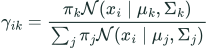
Initialize valid weights, means and covariances. Using the old parameters, compute responsibility γᵢₖ: the posterior fraction of sample i assigned to component k. Each row of responsibilities adds to 1.

LaTeX: \gamma_{ik}=\frac{\pi_k\mathcal N(x_i\mid\mu_k,\Sigma_k)}{\sum_j\pi_j\mathcal N(x_i\mid\mu_j,\Sigma_j)}

Step 3. Use the expected complete-data log likelihood

The “modified” objective in EM is the expectation of the complete-data log likelihood. During this M-step the responsibilities are fixed, so the difficult log of a component sum is replaced by a weighted sum of component log densities.

LaTeX: Q(\theta\mid\theta^{old})=\sum_i\sum_k\gamma_{ik}\left[\log\pi_k+\log\mathcal N(x_i\mid\mu_k,\Sigma_k)\right]

Step 4. M-step: weighted estimates

LaTeX: N_k=\sum_i\gamma_{ik},\quad \pi_k^{new}=\frac{N_k}{N},\quad\mu_k^{new}=\frac{\sum_i\gamma_{ik}x_i}{N_k}

LaTeX: \Sigma_k^{new}=\frac{\sum_i\gamma_{ik}(x_i-\mu_k^{new})(x_i-\mu_k^{new})^T}{N_k}

Repeat E and M until the observed log likelihood changes by less than a chosen tolerance or an iteration limit is reached. EM improves or preserves likelihood under exact steps, but can converge to a local optimum. Try several initializations and avoid singular covariance matrices.

Small responsibility example. If one sample has unnormalized component contributions 0.12 and 0.08, total 0.20 gives responsibilities 0.6 and 0.4. Its mean-update contribution is 0.6x for component 1 and 0.4x for component 2; it is not forced entirely into one cluster. This is why EM is called soft assignment in a GMM.