Intelligent Systems II · TEE · papers
Q5(b) Bike-sharing Markov transitions, retention and gains [10]
Final / re-examination · 28 Apr 2025
Actual historical paper ·100 marks attempted /140 offered · Q1 compulsory + any four of Q2–Q7. Source defects and solution assumptions are explicitly identified.
Around 600 cities globally have bike-share programs where users borrow and return bikes at various stations. The distribution of bikes changes daily as they move between stations. Considering three stations (A, B, C), we can track bike movement from midnight to the next midnight.
- Out of the bikes borrowed from station A,30% are returned to station A,50% end up at station B, and 20% end up at station C.
- Out of the bikes borrowed from station B,10% end up at station A,60% have been returned to station B, and 30% end up at station C.
- Out of the bikes borrowed from station C,10% end up at station A,10% end up at station B, and 80% are returned to station C.
- Develop a Transition Probability matrix
- Interpret the state transition matrix regarding a) Retention & loss b) Retention & gain
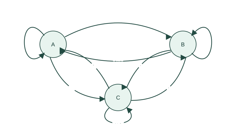
- Draw the State transition diagram
Answer
Given
States ordered A, B, C; one step is one day. The “around 600 cities” sentence is preserved as historical question context, not asserted as a current statistic.
To find
Transition matrix, retention/outflow/inflow interpretation and state diagram.
Formula and why
 LaTeX:
\mathbf n_{t+1}=\mathbf n_tPUse row vectors: rows of P are departure stations, columns arrival stations. Multiplying the initial counts by P gives expected next-day counts. Without starting counts, incoming percentages from different source groups cannot simply be added as a station's probability of gain.
Step 1. Write the transition matrix
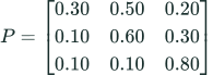 LaTeX:
P=\begin{bmatrix}0.30&0.50&0.20\\0.10&0.60&0.30\\0.10&0.10&0.80\end{bmatrix}Each row sums to 1:0.3+0.5+0.2=1;0.1+0.6+0.3=1;0.1+0.1+0.8=1.
Step 2. Interpret retention and loss from each station
| Origin | Retained at origin | Leaves origin | Where the losses go |
|---|---|---|---|
| A | 30% | 70% | 50% toB;20% toC |
| B | 60% | 40% | 10% toA;30% toC |
| C | 80% | 20% | 10% toA;10% toB |
Step 3. Express retention and incoming gains correctly
Let a, b, c be the starting numbers of bikes. Then:
 LaTeX:
a_{next}=0.30a+0.10b+0.10c LaTeX:
b_{next}=0.50a+0.60b+0.10c LaTeX:
c_{next}=0.20a+0.30b+0.80c| Station | Retained component | Incoming gain from other stations | Net change |
|---|---|---|---|
| A | 0.30a | 0.10b+0.10c | −0.70a+0.10b+0.10c |
| B | 0.60b | 0.50a+0.10c | 0.50a−0.40b+0.10c |
| C | 0.80c | 0.20a+0.30b | 0.20a+0.30b−0.20c |
Whether a station gains bikes overall depends on a, b, c. A column need not sum to 1 because it combines conditional probabilities from different origins.
Step 4. Illustrate only if initial counts are explicitly assumed
For illustration, assume 100 bikes initially at each station. Then next counts areA=30+10+10=50;B=50+60+10=120;C=20+30+80=130. Total remains 300. These initial counts are not printed data.
Step 5. Draw all directed transitions